Mixture Design in the Quantisweb Methodology
M’Hammed Mountassir, Ph.D., Quantisweb Technologies Inc.
Abstract:
This article demonstrates how the Quantisweb methodology, which combines aspects and approaches of three areas of Applied Mathematics: Decision Theory (AHP approach: Analytical Hierarchical Process), Statistics, and Optimization Techniques; is applied in mixtures designs. A comparison study demonstrates that Quantisweb requires 60% fewer experiments to solve the same problem with standard techniques. The acceptable number of optimal parameter value (OPV) combinations using visual RSM techniques in Design Expert and Minitab gives a desirability rate of at least 85% which shows that the procedure is subject to a great degree of variability. Whereas, Quantisweb gives a single optimal combination of parameter values (X) that corresponds to a desired output based upon the product specifications, and the optimization is done analytically, not visually as it is done with standard techniques.
Background to Mixture Design:
In many industries, many products are obtained by mixing several ingredients. The characteristics of these products depend on the proportion of each ingredient in the mixture in question. The k proportions of the components have two important features:
- Their values are non-dimensional numbers and are thus perfectly comparable.
- Their sum is equal to 1 (or 100%), and therefore they are dependent on each other
![]()
The possible field (of feasibility) is a (k-1) simplex. For example, where k=3 ingredients, the experimental field is an equilateral triangle. Where k=4 ingredients, the experimental field is a regular tetrahedron, etc. In these situations, the choice of experiments needs to be carefully determined to allow for proper optimization. That is, some experiments provide more information than others, depending on the method used in the modeling of the characteristics and product optimization.
Since, the large majority of modeling and product optimization methodologies are based on response surface methodology, the experiments should be designed to provide useful information in such frameworks.
Models based on response surfaces:
Generally, when the response surface methodology is used, the characteristics are modeled by m degree polynomials (where m=1, 2, 3, or 4) per the number of k ingredients. To estimate the coefficients of these models, the required number of experiments is ![]() where each ingredient must take the values 0, 1/m, 2/m. …, 1.
where each ingredient must take the values 0, 1/m, 2/m. …, 1.
For example, if k=3 et m=2, the model will be ![]() , where α is the coefficient. For these values of k and m 6 experiments are required. In the case where each ingredient may have the values of either 0, 1/2, or 1, the experimental design may be described as in Table 1:
, where α is the coefficient. For these values of k and m 6 experiments are required. In the case where each ingredient may have the values of either 0, 1/2, or 1, the experimental design may be described as in Table 1:
Table 1: Experimental Design
| Tests | X1 | X2 | X3 |
| 1 | 1 | 0 | 0 |
| 2 | 0 | 1 | 0 |
| 3 | 0 | 0 | 1 |
| 4 | 0.5 | 0.5 | 0 |
| 5 | 0 | 0.5 | 0.5 |
| 6 | 0.5 | 0 | 0.5 |
In the case, where k=3 and m=3, the number of experiments required is 10. Further, where each ingredient may have the values of either 0, 1/3, 2/3, or 1, the experimental design may be as demonstrated in Table 2:
Table 2: Experimental Design
| Tests | X1 | X2 | X3 |
| 1 | 1 | 0 | 0 |
| 2 | 0 | 1 | 0 |
| 3 | 0 | 0 | 1 |
| 4 | 1/3 | 1/3 | 1/3 |
| 5 | 2/3 | 1/3 | 0 |
| 6 | 2/3 | 0 | 1/3 |
| 7 | 0 | 2/3 | 1/3 |
| 8 | 1/3 | 2/3 | 0 |
| 9 | 1/3 | 0 | 2/3 |
| 10 | 0 | 1/3 | 2/3 |
Optimization:
Once each characteristic is modeled, we can proceed to optimization of the mixture. Let us suppose that we have p characteristics Y1,….,Yp to optimize. In the case of mixtures, optimization may be provided using expert systems. Expert systems define desirability functions that we try to satisfy simultaneously for the purposes of optimization. The form of these desirability functions depends on the nature of the optimization desired. For example:
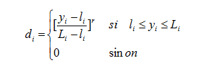
- If the characteristic allows a range of acceptable values
 . The corresponding desirability function is defined by:
- Alternatively, if the characteristic is to be maximized, the desirability function is defined by:
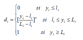
Based on this, the desirability function of all the characteristics to be maximized is ![]() . The maximum of D is that mixture region favorable to all the characteristics, which are here presumed to be of equal importance. If the characteristics do not all have the same importance, this way of simultaneously maximizing characteristics becomes impossible.
. The maximum of D is that mixture region favorable to all the characteristics, which are here presumed to be of equal importance. If the characteristics do not all have the same importance, this way of simultaneously maximizing characteristics becomes impossible.
Mixture-amount designs:
In a mixture-amount problem, each product characteristic depends on the proportions of the different ingredients and on the total quantity of all the ingredients. For example, if we apply different fertilizers to a plot of tomatoes, both the total quantity of the different fertilizers and the proportions of the different fertilizers affect the yield. For example, if we have 3 types of fertilizer and 4 possible quantities for each fertilizer, we must create a design to analyze each of these quantities and try to determine which gives the best yield.
However, the task becomes more complex and difficult if any: of the number of Yj characteristics, the number of Xi parameters, or the number of quantities; per parameter Xi to be evaluated, increases. In fact, the number of experiments required increases exponentially if any of the previous factors increase.
Quantisweb Methodology:
In using the constraints on the parameters of Quantisweb, when there is a standard mixture problem, users have the choice of specifying the (k+1) experiments to perform. Users are free to make the choice they consider the most appropriate, per their experience. Further, other experiments can be added, up to a maximum of 25 total experiments.
Quantisweb can be used to solve a mixture-amount problem in the following way:
- For every quantity to evaluate, a discrete X parameter with modalities (0: Absent, 1: Present) is added, and in using conditional constraints we can ensure that every time only one quantity is present. Therefore, the Quantisweb methodology requires only one additional experiment to evaluate each additional quantity.
- Quantisweb can handle problems of truncated mixtures that treat cases where the sum of the proportions of the ingredients is inferior to the unit, by the simple indication on the constraints. Quantisweb can also handle cases of mixtures of mixtures (c.f. reference [4]).
A Comparison of Mixture Design Using the Quantisweb Methodology and Standard Techniques:
This example is taken from John Cornell’s book Experiments with Mixtures: Designs, Models and Analysis of Mixture Data, (3rd ed.) Wiley Series in Probability and Statistics, 2002.
Standard Techniques:
In this example, there are three ingredients, k=3, and three characteristics, p=3. The author opted for modeling by second degree polynomials (m=2), which normally requires 6 experiments. In addition, he added 4 other experiments inside the simplex, some of which were repeats of the original 6 experiments. For the repeated experiments, the average values of the measured characteristics were taken.
The ingredients were: X1=Fuel; X2= Oxidizer; and X3=Binder. The characteristics were: Y1=Average Burning Rate;
Y2=Standard Deviation of Burn Rate;
Y3=Manufacturability Index.
The data is grouped in the following experimental design matrix found in Table 3:
Table 3: Experimental Design & Result of Experiment
| Test1 | X1 | X2 | X3 | Y1 | Y2 | Y3 |
| E1 | 1 | 0 | 0 | 95.2 | 3.9 | 28.5 |
| E2 | 0 | 1 | 0 | 103.5 | 5.1 | 19.5 |
| E3 | 0 | 0 | 1 | 101 | 13.5 | 15 |
| E4 | 1/2 | 1/2 | 0 | 104 | 6.8 | 20 |
| E5 | 1/2 | 0 | 1/2 | 103.2 | 4.7 | 18 |
| E6 | 0 | 1/2 | 1/2 | 94 | 4.5 | 17 |
| E7 | 1/3 | 1/3 | 1/3 | 104.5 | 3.4 | 19 |
| E8 | 2/3 | 1/6 | 1/6 | 97.1 | 3.5 | 20 |
| E9 | 1/6 | 2/3 | 1/6 | 93 | 5.2 | 22 |
| E10 | 1/6 | 1/6 | 2/3 | 107.2 | 5 | 17 |
Results Reported:
The models of the characteristics were:
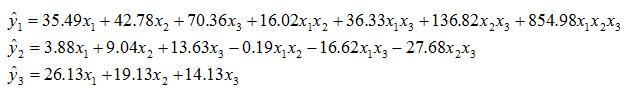
The ideal values of the characteristics were as follows:
![]()
Then, by using Stat-Ease’s Design Expert (1998) and Minitab (1999) software, the authors arrived at 4 acceptable formulations, where the desirability function of the product exceeds 85%. These formulation results were described as shown in the Table 4 below:
Table 4: Formulation results
| Formulation | X1 | X2 | X3 | Y1 | Y2 | Y3 |
| 1 | 0.165 | 0.44 | 0.395 | 104.32 | 4.10 | 18.29 |
| 2 | 0.24 | 0.40 | 0.36 | 104.95 | 4.02 | 19.00 |
| 3 | 0.245 | 0.385 | 0.37 | 105.34 | 4.01 | 18.99 |
| 4 | 0.255 | 0.36 | 0.385 | 105.72 | 4.01 | 19.00 |
Quantisweb Methodology:
With this methodology, only 4 out of the 10 preceding experiments are needed to solve the optimization problem. These experiments are grouped in the Table 5 below:
Table 5: Experimental Values & Result of Experiments
| Tests | X1 | X2 | X3 | Y1 | Y2 | Y3 |
| 1(E5) | 0.5 | 0 | 0.5 | 103.2 | 4.7 | 18 |
| 2(E4) | 0.5 | 0.5 | 0 | 94 | 4.5 | 20 |
| 3(E7) | 0.33 | 0.34 | 0.33 | 104.5 | 3.4 | 19 |
| 4(E6) | 0 | 0.5 | 0.5 | 94 | 4.5 | 17 |
With these experiments, the system indicates that characteristics Y1 and Y2 vary considerably. The models generated are the following:
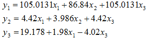
The optimum formulation of the values of the predicted characteristics, where they are given the same importance, is as follows in Table 6 below:
Table 6: Optimum Formulation and Predicted “Y” Values
| X1 | X2 | X3 | Y1(predicted) | Y2(predicted) | Y3(predicted) |
| 0.153 | 0.347 | 0.5 | 98.71 | 4.27 | 17.47 |
To show the flexibility of the Quantisweb Methodology, another choice of the 4 experiments is made. After these 4 experiments, the following data are obtained and shown in Table 7 below:
Table 7: Experimental Values & Result of Experiments
| Tests | X1 | X2 | X3 | Y1 | Y2 | Y3 |
| 1(E2) | 0 | 1 | 0 | 103.5 | 5.1 | 19.5 |
| 2(E1) | 1 | 0 | 0 | 95.2 | 3.9 | 28.5 |
| 3(E7) | 0.33 | 0.34 | 0.33 | 104.5 | 3.4 | 19 |
| 4(E4) | 0.5 | 0.5 | 0 | 104 | 6.8 | 20 |
This set of experiments indicates that all the characteristics are highly variable. The models generated are:
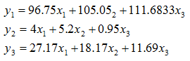
The optimum formulation with the values of the predicted characteristics, where they are once again given the same importance, is as follows and shown in Table 8 below:
Table 8: Optimum Formulation and Predicted “Y” Values
| X1 | X2 | X3 | Y1(predicted) | Y2(predicted) | Y3(predicted) |
| 0.329 | 0.447 | 0.223 | 103.8 | 3.85 | 19.68 |
Now, if the last example is redone and Y1 is made twice more important than the others with Y2 and Y3 kept equal, the optimum formulation obtained is the following found in table 9.
Table 9: Optimum Formulation and Predicted “Y” Values
| X1 | X2 | X3 | Y1(predicted) | Y2(predicted) | Y3(predicted) |
| 0.45 | 0.398 | 0.152 | 102.32 | 4.013 | 21.23 |
Comparative Results Summarized:
The following table 10, summarizes the comparative results based on using both the Quantisweb Methodology and Standard Techniques:
Table 10: Results for Minitab vs. Quantisweb
| Formulation | X1 | X2 | X3 | Y1 | Y2 | Y3 |
| Minitab 1 | 0.165 | 0.44 | 0.395 | 104.32 | 4.10 | 18.29 |
| Minitab 2 | 0.24 | 0.40 | 0.36 | 104.95 | 4.02 | 19.00 |
| Minitab 3 | 0.245 | 0.385 | 0.37 | 105.34 | 4.01 | 18.99 |
| Minitab 4 | 0.255 | 0.36 | 0.385 | 105.72 | 4.01 | 19.00 |
| Quantisweb A | 0.153 | 0.347 | 0.5 | 98.71 | 4.27 | 17.47 |
| Quantisweb B | 0.329 | 0.447 | 0.223 | 103.8 | 3.85 | 19.68 |
| Quantisweb B’ | 0.45 | 0.398 | 0.152 | 102.32 | 4.013 | 21.23 |
Quantisweb A and B
Different experiments and “Yjs” the same weight
Large variability of Y1 and Y2
Quantisweb B’
Weight of Y1 (2 times) that of Y2 and Y3
Large variability of Y1, Y2 and Y3
Conclusion of Quantisweb versus Design Expert (Stat-Ease) and Minitab
- The number of experiments is 10 for Design Expert and Minitab and only 4 for Quantisweb. That is, 60% fewer experiments are required to solve the same problem.
- For Quantisweb based approaches, the addition of the number of “Yj” characteristics and the number of “Xi” parameters has an additive effect on the number of experiments to perform, compared to an exponential effect in traditional methods.
- The Quantisweb method indicates that the characteristics have a large variability.
- The choice of the experiments utilized is flexible with Quantisweb and the OPV generated will be in the optimality region of all the characteristics in the presence of a large variability, or a unique optimum OPV in the absence of a large variability.
- All the “Yjs” have the same importance for Design Expert and Minitab whereas with Quantisweb, the importance of the characteristics can be evaluated based on their values.
- Design Expert and Minitab generate 4 acceptable OPV combinations with a desirability rate of at least 85%. Generating 4 combinations with a visual consensus (RSM) shows that the procedure is subject to a great degree of variability. Quantisweb gives a single OPV combination that is based on a desired output based upon the product specifications, and the optimization is done analytically, not visually.
References:
[1] John Cornell Experiments with Mixtures: Designs, Models and Analysis of Mixture Data, (3rd ed.). Wiley Series in Probability and Statistics, 2002.
[2] Jean-Jacques Droesbeke & al. “Plans d’experiences, applications a l’entreprise”. Editions technip, Paris, 1997.
[3] Draper, N.R. and R.C. John: “A mixtures model with inverse terms” Technometrics, Vol. 10, pp. 37-46 (1977).
[4] Mountassir, M. “An Innovative Methodology in the Area of Formulation”, White paper, MDM Technology Inc, 2006.